For a linear or straight line function, Linear Least Squares Curve Fitting we want to find the function,
f (x) = mx + c
which most closely fits our data points. That is, for a linear graph we need to discover the gradient m and the intercept c which gives this best fit to our data. Firstly we assume our values of the independent variable x have no error (or negligible error) but that the dependent variable y may have an appreciable random scatter.
An individual data point (xi, yi) has a residual, R, which is defined as the difference between the experimental data yi and the value of yi that is predicted by the model equation straight line, y, = mx, + c
R = y, – (mx, + c)
Removing the bracket the residual is,
R= Y,— mx, – c
We take the square of the individual residuals, SR, to give equal weight to those data points which lie above the predicted line and those that lie below the line predicted of the model equation.
SR = (y,— mx, – c)^2
We take the sum the square of the residuals, SSR, of each of the data points to give an overall picture of the scatter of all the n data points. The sum of square of all the residuals SSR is,
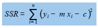
where n = number of data points. We will obtain the best fit for a straight line graph by minimizing the value of the sum of squares of the residuals by varying the values of xi and c, hence the common name of a “least square” fit. This best fit line is called the linear least squares (LLSQ) line. The easiest way of curve fitting of equations to experimental data is to use a spreadsheet. You can use LibreOffice Calc, or OpenOffice Calc, which are both open-source and free, or Microsoft Excel, see the References. In Calc or Excel you use an array function called LINEST (lin est) to fit a linear equation.
The LINEST algorithm works by an iterative process. It increases m by a small amount and then decreases m by the same small amount. It then compares the original SSR with these two altered values and chooses the value for m which leads to the smallest of these three SSR values. Holding this value of m constant for the moment, the algorithm then alters the intercept c by increasing and decreasing it and choosing the value of c which gives Ihe smallest of the resulting three SSR values. LINEST then keeps repeating the above pair of cycles for the two variables until the final value of SSR is only changing by an insignificant amount. Let us look at a worked example as the best way of seeing how Linear Least Squares curve fitting works.